CastorisCausa

When multiple statistical comparison are simultaneously performed, the risk of discovering false statistical significance increases as the number of comparisons increases. As such, Bonferroni correction is a commonly used method to address this multiple comparisons problem. In this post provides a visual demonstration to show why the multiple comparison problem is presented and needs to be addressed. The demonstration is based on theoretical and experimental results, and with it I hope the multiple comparisons problem will look more intuitive and understandable. All the codes to generate the results and figures in this post can be found here.

Comparing groups

Let's have two populations or random variables (RV) \(X\) and \(Y\). We want to evaluate if the means of these populations are significantly different. In other words, we want to perform an hypothesis test to determine if there is a significant difference between their means which are \(\mu_X\) and \(\mu_Y\) respectively. In most of the cases, there is not have access to all the realizations of the RVs, as such the hypothesis test is performed with statistical samples (data) that are obtained by sampling the RVs, this is to say, by performing an experiment. Two hypothesis are considered: one null hypothesis \(H_0\) (there is no difference between means), and one alternative hypothesis \(H_1\) (there is difference between means), these are formulated as:

1. \(H_0\): \(\mu_X = \mu_Y\) or \(\mu_X - \mu_Y = 0\)
2. \(H_1\): \(\mu_X \neq \mu_Y\) or \(\mu_X - \mu_Y \neq 0\)

It is concluded that there is a significant difference in the population means, \(H_0\) is rejected, if there probability of having a difference between means at least or larger than the observed from the data is smaller than the significance level or \(\alpha\). Otherwise, \(H_0\) is NOT rejected based on the available data. A commonly used value for \(\alpha\) is 0.05 (this is to say 5%).

To demonstrate the effects of multiple comparisons, the same the same hypothesis test will be tested in two scenarios:

1. One comparison: \(X\) and \(Y\) are described as univariate or single RV.
2. Two or more comparisons: \(X\) and \(Y\) are described as multivariate RV.

Note: when \(n\) sample points are obtained from a normal distributed RV \(W\), we obtain the sample \(w\) which consists of \(n\) realizations of \(W\). If \(n\) is large, usually above 30, by the Law of Large Numbers (LLN) the mean of \(w\) or sample mean (\(\bar{w}\)) is a good estimation of \(\mu_W\). Also for large values of \(n\), again usually over 30, the standard deviation of \(w\) or sample standard deviation (\(s_w\)) is a good estimation of the standard deviation of the population (\(\sigma_W\))

1. One comparison

To begin, let's assume the \(H_0\) is true, there is no difference between \(\mu_X - \mu_Y\). Indeed, let's assume that \(X\) and \(Y\) follow the same distribution, the standard normal distribution \(\mathcal{N}(\mu=0,\sigma^{2}=1)\).

To test the difference between the population means, were are interested in the sampling distributions of the sample means. Thus, let's consider two new RVs: \(\bar{X}\) and \(\bar{Y}\), which are the sampling distribution of the sample mean for the populations \(X\) and \(Y\) respectively. The mean and standard deviation of these sampling distributions of the sample means are: \(\mu_\bar{X} = \mu_X\) (remember that \(\mu_X = \bar{x}\)), and \(\sigma_\bar{X} = \sigma_X/n\) (remember that \(\sigma_X = s_x\)). The same goes for \(\mu_\bar{Y}\) and \(\sigma_\bar{Y}\).

Now, lets have another RV called \(Z = \bar{X} - \bar{Y}\). As \(\bar{X}\) and \(\bar{Y}\) are normally distributed, \(Z\) is also normally distributed with \(\mu_Z = \mu_\bar{X} - \mu_\bar{Y}\) and \(\sigma^2_Z = \sigma^2_\bar{X} + \sigma^2_\bar{Y}\). See link.

The difference in \(\mu_X\) and \(\mu_Y\) will be considered significant if it has an occurring probability of 5% or less. As such from the normal distribution of \(Z\), we can identify the standard score (or z-score) for this probability, this means that the difference is significant when is absolute value is larger than \(1.96\sigma_Z\). As 95% of the values are between -\(1.96\sigma_Z\) and \(1.96\sigma_Z\).

Probabilities and standard scores for normal distribution.

All this is to say, just by chance there is a probability of 5% or less that the absolute difference between \(\mu_X\) and \(\mu_Y\) is larger than \(1.96\sigma_Z\). To verify this in the simulation, 10,000 samplings were done to \(X\) and \(Y\), each sample consisting in 100 sample points. The graph below presents the theoretical probability density function (pdf) for \(Z\), and the empiric pdf obtained from the simulation.

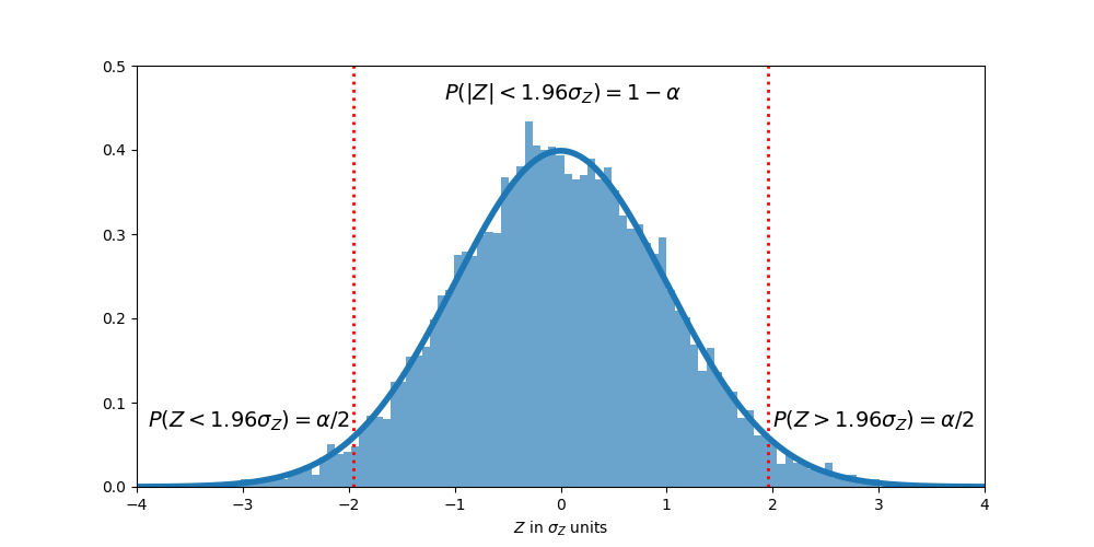
Probability distribution for \(Z\). Solid line: theoretical results. Shaded area: simulation results.
Theoretical: \(P(|Z|>1.96\sigma_Z) = 0.05\)
Experimental: \(P(|Z|>1.96\sigma_Z) = 0.0475\)

So far so good, the null hypothesis is rejected around 5% of the time. But the problems start with multiple comparisons.

2. Two or more comparisons

Again, let's assume the null hypothesis is true. Thus, in this scenario, each population (\(X\) and \(Y\)) is characterized by a set of two independent RVs, which have a standard normal distribution. As the variables are independent and normally distributed, the covariance matrix for \(X\) and \(Y\) is a diagonal full with the variance of variable, in this case 1. This is to say:

• \(X = [X_1, X_2],\) with \(X_1\sim \mathcal{N}(\mu_{X_1}=0,\sigma_{X_1}^{2}=1)\) and \(X_2\sim \mathcal{N}(\mu_{X_2}=0,\sigma_{X_2}^{2}=1)\)
• \(Y = [Y_1, Y_2],\) with \(Y_1\sim \mathcal{N}(\mu_{Y_1}=0,\sigma_{Y_1}^{2}=1)\) and \(Y_2\sim \mathcal{N}(\mu_{Y_2}=0,\sigma_{Y_2}^{2}=1)\)

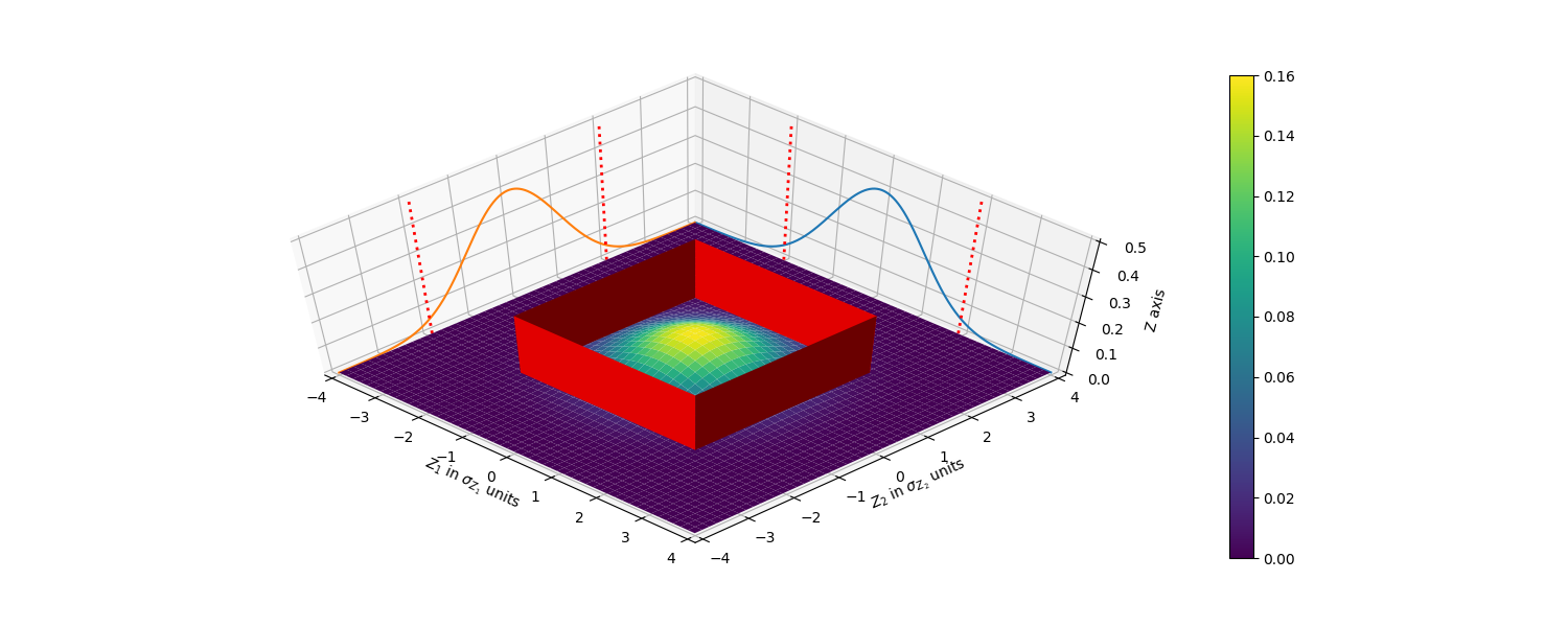
Let's follow the same approach as in the one-comparison section for each of the two comparisons: \(X_1\) vs \(Y_1\) and \(X_2\) vs \(Y_2\). Let's define a third bivariate RV, \(Z = [Z_1, Z_2]\) with \(Z_1=X_1-Y_1\) and \(Z_2=X_2-Y_2\). A difference in means would be considered significant if it has an occurring probability of of 5% or less; this means that the difference is significant when \(|Z_1| > 1.96\sigma_{Z_1}\) OR \(|Z_2| > 1.96\sigma_{Z_2}\). The figure below shows the pdf of \(Z\), with the marginal pdf for \(Z_1\) and \(Z_2\).

pdf of \(Z\), marginal pdf for \(Z_1\) with \(\pm1.96\sigma_{Z_1}\) indicated as dotted red lines, and pdf for \(Z_2\) with \(\pm1.96\sigma_{Z_2}\) indicated as dotted red lines.

The pdf for \(Z\) is a surface where the total volume under the surface is equal to 1. By analyzing the pdf of Z and the marginal pdfs for \(Z_1\) and \(Z_2\), we can see that the box inside the red walls represents the probability that \(|Z_1| < 1.96\sigma_{Z_1}\) AND \(|Z_2| < 1.96\sigma_{Z_2}\), as \(Z_1\) and \(Z_2\) are independent, this can be written as:

\(P(Z\) is inside red box\()\) = \(P(|Z_1| < 1.96\sigma_{Z_1})\) \(P(|Z_2| < 1.96\sigma_{Z_2})\)

\(P(Z\) is inside red box\()\) = \(0.95*0.95 = 0.9025\)

This result can be rephrasing as: finding a significant result in \(Z_1\) OR \(Z_2\), is equal to 1 minus the probability of not finding a significant results for \(Z_1\) nor for \(Z_2\). Then the problem the multiple simultaneous comparisons is evident, as there is a probability of 9.75% of finding a significant result in \(Z_1\) or \(Z_2\) just by chance. Which is higher to the 5% probability deduced in the one comparison case. This is extended for \(m\) multiple comparisons as:

\(P\)(finding at least one significant result\() = 1 - (1-\alpha)^m\)

The possibility of rejecting the null hypothesis, or finding a significant results just by chance, gets larger the more comparisons are performed simultaneously.

To address this problem, a common method used is Bonferroni correction. In this method, the significance level is adjusted to compensate for the increment in the probability of finding at least one significant result. As such the corrected significance level is \(\alpha/m\) for a desired significance level \(\alpha\) in \(m\) multiple comparisons.

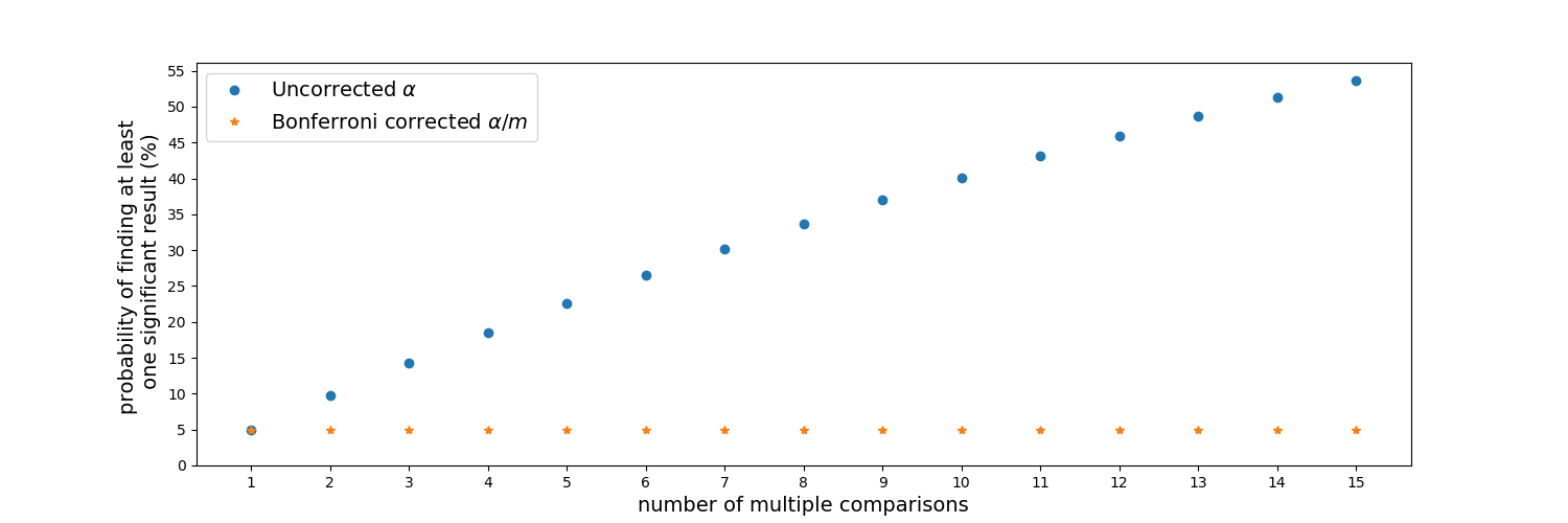
Probability of finding at least one significant result. Uncorrected and Bonferroni-corrected for multiple comparisons.

Getting back to the bivariate RV, the regions obtained by using the significance level \(\alpha\) or \(\alpha/m\) are shown below. The standard score (or z-score) for the corrected significance level \(\alpha/m\) is 2.24. Moreover, the theoretical results are compared with the one from the simulation, where 10,000 samplings were done to \(X\) and \(Y\), each sample consisting in 100 sample points.

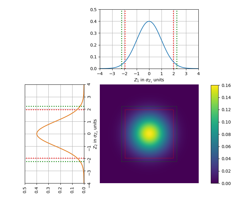
pdf of \(Z\), marginal pdf for \(Z_1\) with \(\pm1.96\sigma_{Z_1}\) indicated as dotted red lines and \(\pm2.24\sigma_{Z_1}\) indicated as dotted green lines; and pdf for \(Z_2\) with \(\pm1.96\sigma_{Z_2}\) indicated as dotted red lines and \(\pm2.24\sigma_{Z_2}\) indicated as dotted green lines.
Theoretical: \(P(Z\) is outside red box\() = 0.0975\)
Theoretical: \(P(Z\) is outside green box\() = 0.05\)

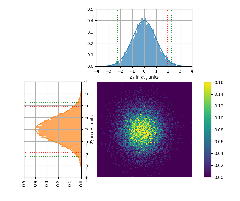
pdf of \(Z\), marginal pdf for \(Z_1\) with \(\pm1.96\sigma_{Z_1}\) indicated as dotted red lines and \(\pm2.24\sigma_{Z_1}\) indicated as dotted green lines; and pdf for \(Z_2\) with \(\pm1.96\sigma_{Z_2}\) indicated as dotted red lines and \(\pm2.24\sigma_{Z_2}\) indicated as dotted green lines.
Experimental: \(P(Z\) is outside red box\() = 0.1053\)
Experimental: \(P(Z\) is outside green box\() = 0.0552\)

I hope this post helps to understand better why it's important to take action when multiple comparisons are performed.

References

• Multiple comparisons problem
• hy is multiple testing a problem?
• Bonferroni correction
• Normal distribution
• Central limit theorem
• Comparison of Two Means
• Unbiased estimation of standard deviation
• Comparing two means
• Sampling distribution
• Standard normal distribution, Z-score table
• Point estimation of the mean